
 Abstract
- There are several established methodologies for generating synthetic populations. These include deterministic reweighting, conditional probability (Monte Carlo simulation) and simulated annealing. However, each of these approaches is limited by, for example, the level of geography to which it can be applied, or number of characteristics of the real population that can be replicated. The research examines and critiques the performance of each of these methods over varying spatial scales. Results show that the most consistent and accurate populations generated over all the spatial scales are produced from the simulated annealing algorithm. The relative merits and limitations of each method are evaluated in the discussion.
- Keywords:
- Conditional Probability; Deterministic Reweighting; Population Synthesis; Simulated Annealing; Spatial Scales
Introduction
- 1.1
- Recent years have seen a rise in the number of methods and applications that require realistic individual-level data/synthetic populations. This trend can be attributed to a number of factors including increases in computational power and storage, a wealth of individual level data (for example, the British Household Panel Survey) and the development of new computational paradigms, such as cellular automata and agent-based modelling (ABM).
- 1.2
- Static spatial microsimulation creates a synthetic population (a population built from anonymous sample data at the individual level) which realistically matches the observed population in a geographical zone for a given set of criteria. There is a diverse set of research and policy applications that use synthetic populations in a spatial setting, including: health (Brown & Harding 2002; Smith, Pearce, & Harland 2011; Tomintz, Clarke & Rigby 2008), transportation (see, for example, Beckman, Baggerly ,& McKay 1996; McFadden, Cosslett, Duguay, & Jung 1977) and water demand estimation (Williamson & Clarke 1996).
- 1.3
- ABM can also use synthesised data as a base population. There has been a rapid uptake in the use of ABM in Geography (see Heppenstall, Crooks, See, & Batty 2012 for a detailed discussion) with applications ranging from simulating the movement of burglars (Malleson, Heppenstall, & See 2010) to replicating dynamics in spatial retail markets (Heppenstall, Evans, & Birkin 2006). Although the construction of an ABM does not require a complete individual data set, creating an agent population from a comprehensive realistic synthesised individual dataset can only improve the realism of these models.
- 1.4
- The accuracy and realism with which differences in populations within geographical areas are captured may have great significance for modelling, especially where the results are used to inform policy. The UK Census collects a vast array of data at individual level, but for issues of confidentiality data are aggregated to larger geographic scales. The coarser the geographic scale at which census data is published, the more attribute detail can be accessed. However, at fine geographical scales (for example, output areas with average populations of about 300) detailed population attributes are not available. This has led to research focused on creating synthetic populations that represent a population realistically within a predefined geographical area, simulating combinations of attributes not disclosed within Census data, effectively filling in the blanks.
- 1.5
- There are several established methodologies for generating synthetic populations. The focus of this paper will be on spatial microsimulation techniques, specifically: deterministic reweighting (Smith, Clarke & Harland 2009; Smith et al. 2011), conditional probability (Monte Carlo simulation) (Birkin & Clarke 1988, 1989) and simulated annealing (Openshaw 1995; Voas & Williamson 2000, 2001; Williamson, Birkin, & Rees 1998). These methods were selected due to their common application in geography. Many recent spatial microsimulation studies including Anderson (2007), Ballas et al. (2005), Morrissey, Clarke, Ballas, Hynes, and O'Donoghue (2008), Smith et al. (2009), Tomintz et al. (2008) and Voas and Williamson (2000, 2001) and have adopted a variation on at least one of the three approaches examined here.
- 1.6
- The aim of this paper is to critically and systematically evaluate the accuracy of the three static spatial microsimulation methods in replicating real-world small-area populations. Outputs from each method are assessed using a measure of absolute error calculated by comparing the estimated population against the population reported in the Census. The model outputs include the following sets of estimates: 1) Census population characteristics used to create the synthetic populations (constraint variables), 2) cross-tabulation of the constraint variables and 3) outputs of variables that available from the Census but are independent of the constraint variables. Each set of outputs from the three models is tested for error, and the results compared to identify the most accurate microsimulation method of synthetic population generation. In addition, the work within this paper critically compares each approach at three different spatial scales, extending the initial work reported in Voas and Williamson (2000, 2001).
- 1.7
- We are unaware of any previous attempts to comprehensively test multiple synthetic population estimation methods. The research of Voas and Williamson (2001) examined the performance and appropriateness of different evaluation statistics for use when synthesising populations. Recommendations from this research will be incorporated and extended here. Voas and Williamson (2000) did not assess the viability or performance of alternative population synthesis techniques (using combinatorial optimisation to produce their synthetic populations) or the effects of different spatial scales on population synthesis algorithms.
Spatial microsimulation algorithms
-
The modelling approach
- 2.1
- The approach can be stated generically as follows. We begin with a population of individuals termed the sample. The sample relates to a higher level region, such as a country or one of its statistical areas, and for these regions we aim to simulate the population of its constituent small areas. To do this, weights will be applied to each member of the sample. For example, if the small area is close to a university then we might wish to apply high weights to members of the sample who are young adults or students; on the other hand, if the area is multi-ethnic then the largest weights might be for residents whose country of birth is outside the UK. For each small area we have a series of constraining tables, or simply constraints, which count the distribution of characteristics in the population for a range of attributes[1]. The objective of the simulation model is to generate a set of weights so that when the sample population is aggregated, the goodness of fit between the model distributions and the equivalent constraints is maximised. A mathematical expression of the problem is given in Appendix A.
- 2.2
- In this paper, we will consider three methods for the optimisation of the population synthesis/microsimulation model — deterministic reweighting; conditional probabilities; and simulated annealing. We use constraining tables for six constraints — gender, ethnic group, age, marital status, socio-economic group, and educational qualifications. Data is extracted from the 2001 census of population at three levels of aggregation (see below, ¤3.3 and $5.1).
Deterministic Reweighting
- 2.3
- The deterministic reweighting algorithm was introduced by Ballas et al. (2005) and has been widely used in microsimulation models for healthcare research. As described by Smith et al. (2009) this algorithm proportionally fits each individual record in the sample population to the observed counts in each of the constraint tables iteratively until each of the constraints have been included.
- 2.4
- In the deterministic reweighting procedure, we start with the first constraint and weight each individual record in the sample. For example, if the first constraint is gender and there are 10,000 males in the sample and 100 males in the small area, then every record in the sample which represents a male will be weighted at 100 / 10,000 = 0.01. Next, we use the weights derived for attribute 1 and we repeat the process for attribute 2. For example, if the second constraint is age and the small area is a community with many elderly residents, then the weights for young people in the sample will be reduced. The process is repeated for each of the constraints iteratively. (see Appendix B).
- 2.5
- However, perfect matching between the synthetic totals and sample totals from the reweighting algorithm cannot be reached for every geographical zone. The more dissimilar the characteristics of an area are from the distribution of characteristics in the sample population the greater the resulting error, as this method assumes all of the areas are relatively homogeneous. A zone with a high ethnic minority population will differ to the average distribution of ethnic minority groups in the sample population, making such a zone less likely to match the constraint table perfectly. One method to minimise the error resulting from the assumption of homogeneity is to run the reweighting algorithm using only the geographic areas which are most similar in terms of population constraints; this can be accomplished by running a cluster analysis in a statistical package such as SPSS to 'group' the most similar geographic areas together (Smith et al. 2009; Smith et al. 2011). This approach is used within this work. If the model is run with the areas which have a similar ethnic makeup (for example) in one set, then the results will be more accurate. Despite this algorithm having no stochastic element and being completely deterministic, the order in which constraints are applied can produce different resulting populations as each new weight produced is a product of the weight calculated using the preceding constraint information. Initial experimentation showed that it was best to order the constraints in such a way that the strongest predictor of an outcome (social class is a strong predictor of obesity, as this method is often used in health applications) is reweighted against the known population first. The DR algorithm is expressed mathematically in Appendix B.
Conditional Probabilities
- 2.6
- The conditional probabilities model is an adaptation of the synthetic estimation procedures first introduced by Birkin and Clarke (1988). A feature of the conditional probabilities model is that the model population is itself synthetically derived and is built up constraint by constraint in accordance with underlying probabilities from the sample population, rather than being reweighted from that sample. As in the previous method (deterministic reweighting) each constraint is considered in turn. For each small area, a synthetic record is created for each individual. Let us suppose the first constraint is gender, as before. The characteristic of 'male' or 'female' is added to each individual in accordance with the associated constraining table. However in this case, the assignment of characteristics is stochastic rather than deterministic. Let us suppose that 60% of individuals are male (in a given area). For each individual, a number between zero and one is pulled from a random distribution and if this number is less than or equal to 0.6 then the individual is assigned the characteristic 'male'; otherwise it is assigned as 'female'. This approach is commonly referred to as 'Monte Carlo sampling'.
- 2.7
- For the second attribute, for example age, the probabilities depend on the constraint (gender) which has already been established. Hence if male individuals are typically older than female individuals then the probabilities will be adjusted accordingly. The data for these conditional probabilities is drawn from observed data in the SAMs (Sample of Anonymised Records). However these probabilities also need to be adjusted in accordance with the constraining table for the new variable (age). We proceed by Monte Carlo sampling for all individuals as in the previous step, and when ages have been assigned to every individual the distribution is summed for the whole area and compared to the constraining table. Now the individual probabilities are weighted — for example, if there are too many people in the age group 20-24 for this small area, then these probabilities are all adjusted downwards. The procedure is repeated iteratively until a close match is achieved with the constraining table. Convergence to the constraints has usually been found to be rapid and robust, and in the examples which we introduce below no special measures have been taken to ensure that this procedure is well-behaved.
- 2.8
- The method continues in the same way for the remaining attributes. As the number of constraint increases, then the conditional probabilities become more elaborate. Here we have six constraints, so at the final step in the procedure then we will have conditional probabilities of the form:
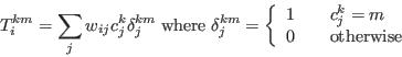
P (qualification | gender, age, ethnicity, marital status, socio-economic group) - 2.9
- As with deterministic reweighting, the order in which constraint are introduced to this model is significant. For optimal results it makes sense to start the constraint with relatively low entropy distributions in which the populations is relatively evenly distributed between the categories — for example gender and age, rather than ethnicity or qualifications, where the number of people of Asian backgrounds or with postgraduate qualifications may be quite small in many areas. However capturing the best predictor variables early in the process is also paramount. For example, if qualifications vary widely by ethnicity, ethnicity should be estimated before qualifications. The experiments presented within this paper show this procedure to be effective, however further improvements are possible by changing the order of constraint selection in the model.
- 2.10
- In earlier versions of the synthetic estimation process in which individual sample data has not been available (e.g. Birkin & Clarke 1988, 1989; see also Beckman et al. 1996) it has been necessary to estimate compound probability distributions using iterative proportional fitting. In essence, this method involves combining partial estimates — for example, we know qualifications by gender and age; qualifications by gender, ethnicity and marital status; and qualifications by gender, age, and socio-economic group. These need to be combined to provide a best estimate of qualifications by gender AND age AND ethnicity AND marital status AND socio-economic group and IPF is a way to achieve this. In the model we present here no iterative proportional fitting is required because full distributions can be extracted from the micro-data.
- 2.11
- With each additional constraint, the synthetic estimation procedure becomes increasingly difficult to implement. In particular, when the number of constraint and associated characteristics is large then the compound probability matrix will become very sparse. In this situation it may be necessary to make further judgements about which attributes are most strongly linked so that those which are less important can be excluded from the estimation process. On the other hand a great strength of this approach is that it can be used to combine micro-data from multiple sources (although this feature is not exploited in the comparative examples presented later in this paper). For example, the synthetic population could be extended to include attitudes or lifestyle behaviour from a source such as the British Household Panel Survey or Family Spending. An early illustration is the generation of synthetic income estimates for small areas (Birkin & Clarke 1989).
- 2.12
- It is clear that deterministic reweighting and conditional probabilities differ in a number of fundamental ways. As the name suggests, deterministic reweighting is a deterministic technique, while conditional probabilities relies on stochastic choices using Monte Carlo selection. Deterministic reweighting is based on reweighting a survey sample, while conditional probabilities establishes a synthetic population using probabilities derived from the underlying sample. Estimation of the conditional probabilities model is a sequential process in which each attribute is created in a single step, whereas deterministic reweighting is an iterative process in which the weights associated with each attribute and the associated constraints are continuously refined. Further comparisons of these techniques with simulated annealing are discussed in ¤2.16. The conditional probabilities algorithm is mathematically expressed in Appendix C.
Simulated Annealing
- 2.13
- Finally, "Simulated annealing is stochastic computational technique derived from statistical mechanics for finding near globally-minimum-cost solutions to large optimisation problems" (Davies 1987). In this application, we take a sample and assume that this is large relative to the population of a small area which is to be modelled. The problem is to extract a subset from the sample which provides the best possible match to the small area population. In other words, the weights on the individual members of the sample are either one (if the individual is selected) or zero (if the individual is excluded). The essence of the procedure is to start by creating a population as a random extract from the sample file, and by aggregating for the various constraints, the goodness of fit of the population to the constraining tables can be evaluated. From this population, we now select an individual member at random, and we consider replacing it with another individual which is also selected at random from the sample population. The aggregation and goodness of fit evaluation is repeated and if the fit is improved then the new individual replaces the old.
- 2.14
- The feature which distinguishes simulated annealing, for example in contrast to hill-climbing algorithms, is the incorporation of the Metropolis Algorithm allowing both backward and forward steps to be taken when searching for an optimal solution (Otten & van Ginneken 1989). So even if the replacement leads to deterioration in the model fit it will be allowed by the model as long as a certain threshold is exceeded. This threshold is often characterised as a 'temperature' step—or annealing factor—as this method was originally conceived as a means to simulate the annealing process by which metals are cooled. As the algorithm proceeds, the (temperature) thresholds are reduced and so backward steps become progressively more unlikely, so that ultimately only climbing moves are permitted towards an optimised outcome.
- 2.15
- Simulated annealing is similar to deterministic reweighting to the extent that weights are applied to members of a sample population. However in simulated annealing these weights are zero-one representing selection or exclusion, whereas in deterministic reweighting the weights are fractional. SA is a heuristic hill-climbing algorithm rather than an iterative process (deterministic reweighting) or sequential estimation method (conditional probabilities). One of the most important differences is that simulated annealing evaluates individual moves simultaneously against all of the constraining tables whereas in both of the other techniques this evaluation takes place constraint by constraint. The simulated annealing algorithm is expressed mathematically in Appendix D.
Comparison of Techniques
- 2.16
- Table 1 shows a summary of some of the important characteristics to be considered when selecting an algorithm to use for each of the algorithms discussed in this section. The first point considered is the ease of setup; how much pre-processing is required to obtain a robust fit-for-purpose output? As both the deterministic reweighting and conditional probabilities algorithms reweight the resulting populations using one constraint at a time, building on the results from the previous constraint, they are sensitive to the constraint order specified within the model. In order to ensure that the output from these two algorithms is suitable, pre-processing analysis is required to ensure an optimal constraint order specification. This may be done using regression analysis to identify the strongest predictor of a particular outcome, for example social grade for smoking behaviour (Tomintz et al. 2008), and ordering the constraints accordingly. In this paper, deterministic reweighting does not use joint probabilities in the reweighting process, although this is an option when using conditional probabilities.
- 2.17
- The primary difference between deterministic reweighting and conditional probabilities is the lack of a stochastic process in deterministic reweighting. Because the deterministic process will give the same result every time, the impact of slight modification to the constraint variables will be clear from the results. For instance, if the prevalence of type 2 diabetes is modelled using a deterministic method and the researcher wishes to estimate the impact of an aging population on diabetes prevalence, the age constraint may be shifted to reflect an older population and the model re-run to estimate diabetes prevalence under this aged population distribution. In contrast, the simulated annealing algorithm places equal weight on each constraint (although this can be changed at the researcher's discretion) and thus the constraint order is of no consequence to the outputs.
- 2.18
- The number of constraints that can be specified is related to the speed of execution of each algorithm. The deterministic reweighting algorithm reweights the sample population using all of the constraint information in a specified order. As more constraints are added, the difference in sample population and constraint frequency distributions can become more pronounced, especially at finer geographies where constraint populations are small. Therefore, less robust results may be produced as additional constraints are included in the model. The conditional probabilities model suffers with similar issues; however these are less pronounced due to the joint probabilities for constraint combinations being adjusted in isolation. However, increasing the number of constraints increases both the processing time and the likelihood of being unable to converge on a suitable joint probability for a constraint combination. Simulated annealing also suffers from a time performance penalty as the number of constraints is increased although the rate increase is less severe than for the other two algorithms.
- 2.19
- One of the major advantages that the conditional probabilities method has over the other two algorithms is that if a sample population is unavailable, a synthetic population can be created using only the aggregate information from the constraint tables. However, as the algorithm here requires a sample population from which to extract the initial joint probabilities, an alternative source for this information is required in the absence of a sample population otherwise erroneous individuals, such as married children, could be produced. A major advantage of the simulated annealing approach, as discussed above, is the inclusion of the Metropolis Algorithm. However, the drawback to added search power is the associated higher computational times. Neither the conditional probabilities method nor the deterministic reweighting method can take backwards steps when searching for a solution.
- 2.20
- Finally, both the conditional probabilities and the simulated annealing methods contain a stochastic element that results in the creation of a different population configuration each time the model is run. This allows the model to consider and produce alternative and potentially more realistic populations. Deterministic reweighting does not have this capability. However, because deterministic reweighting produces the same result with each model run, the impacts of any starting constraint change is more easily quantifiable and can be important for policy evaluation, as discussed above.
Table 1: Summary comparison of the three algorithms Deterministic Reweighting Conditional Probabilities Simulated Annealing Easy setup (is there much pre-processing)? Yes Yes No Sensitive to specification of constraint order? Yes Yes No Limit to number of constraints that can be used? Yes Yes No Requires a sample population? Yes No Yes Can take forward and backward steps to find an appropriate solution? No No Yes Stochastic? No Yes Yes Speed of execution Fastest Middle Slowest
Experiment Set Up
- 3.1
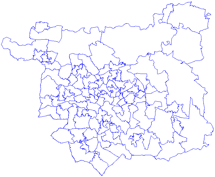
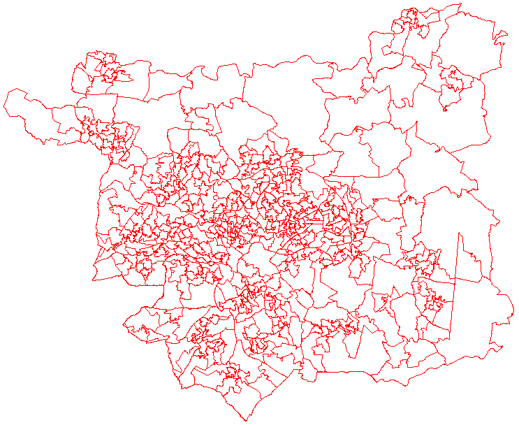
- This experiment will be conducted using the study area of Leeds (UK) Metropolitan District Area (MDA), Figure 1. The population of the Leeds MDA in the 2001 Census was 715,402. The city has two universities leading to areas with high student numbers, a diverse ethnic community with high concentrations of ethnic minority groups in some areas, a large all male gaol with a capacity of 1,004 inmates and several sparsely populated industrial zones. There are two main reasons for choosing this study area. Firstly, the geographical diversity should prove a challenging test for the algorithms making strengths and weaknesses more apparent. The second is the authors' familiarity with the area, allowing any discrepancies in results to be examined in the context of the specific geographical area and its known characteristics.
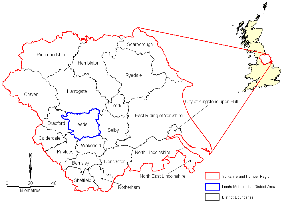
Figure 1. Location of Leeds Metropolitan District Area - 3.2
- Each of the spatial microsimulation methods discussed is used to produce a synthetic population at the Output Area (OA), Lower Layer Super Output Area (LLSOA) and Middle Layer Super Output Area (MLSOA) spatial scales. OA is the finest geography for which Census 2001 data is available with 2,439 in the Leeds MDA each consisting of a population of approximately 300. LLSOA are the next geographical level aggregated from OAs, therefore the 2,439 Leeds OAs nest completely within the 476 Leeds LLSOAs. MLSOAs are the coarsest geography used in this work and are an aggregation of LLSOAs; both the Leeds OAs and LLSOAs will nest completely within the 108 Leeds MLSOAs (see Appendix E for maps showing each geography within the case-study area). The synthesised populations are tested against known Census information, produced at all three geographies OA, LLSOA and MLSOA, to evaluate each algorithmic approach. While we aggregate to evaluate at different geographical scales, the data itself is not aggregated, i.e. the individuals are placed into the aggregated geographies. In summary, each population produced will be tested to examine:
- Reproduction of variables used to constrain each of the synthetic models at each of the different spatial scales.
- Evaluation of the populations produced against information extracted from the Census of Population 2001 using the constraint variables cross-tabulated against each other.
- Examination of how reliably information from the sample population not included in the model constraints can be captured.
- Aggregation of outputs from OA to LLSOA and MLSOA and a subsequent evaluation of the aggregated output against Census of Population 2001 at the appropriate geographical level.
Data
- 3.3
- As discussed previously, the sample population is typically 'sample based' and this research uses the relevant SAMs file extract for the Leeds MDA. The SAMs file for Leeds contains 35,986 anonymised individual resident records intended to represent the actual population of the district in distribution and characteristics.
- 3.4
- The sample population is used alongside aggregate real world data (for both attribute and spatial area) extracted from the 2001 Census. These data will be used as six single attribute (univariate) constraints incorporated into all model runs to assist in the production of each synthetic population (Table 2). For the evaluation of the resulting synthetic populations the univariate constraint attributes have been extracted from the census information as cross-tabulated data (Table 2). These cross-tabulated data provide the necessary information to enable the evaluation of information capture relating to the relationships between the univariate constraint data. To assess how well information is captured outside of the constraint attributes the univariate variables Tenure of Accommodation and Limiting Long Term Illness and cross-tabulated attributes Gender by Hours Worked and Economic Activity by Car (Ownership) are used.
Table 2: Summary of constraint and validation variables Variable Census Table Constraints Gender KS001 Ethnic Group KS006 Age KS002 Marital Status KS004 NSSEC KS014a Highest Qualification KS013 Validation/Evaluation Gender by Age CS002 Marital Status by Age CS002 Gender by Marital Status by Age CS002 Gender by Ethnicity CT003 Age by Ethnicity CT003 NSSEC by Age CS042 NSSEC by Highest Qualification CS114 Tenure of Accommodation CS017 Limiting Long Term Illness KS021 Gender by Hours Worked CS038 Economic Activity by Car Ownership CS061 Table abbreviations - KS: Key Statistics, CS: Census Area Statistics, CT: Census Area Statistics Theme Tables Data Preparation
- 3.5
- A disclosure control measure was applied to the 2001 Census of Population in England called the Small Cell Adjustment Method (SCAM) (Stillwell 2002). Census tables containing categories with small counts (less than 3) have been adjusted. Therefore, the overall totals in different tables do not necessarily sum to the same number for the same geographical area. Although the algorithms applied here do have the ability to cope with small discrepancies in table totals, the associated 'noise' introduced by SCAM may influence the resulting output. It is not the intention of this paper to test how well each algorithm can handle the discrepancies in the data, but to test how well they manage to produce a realistic synthetic population.
- 3.6
- Therefore the information extracted from the census has been adjusted to ensure that each table used to constrain or evaluate the models sum to consistent population totals for each zone, and that the sum of all zone populations equals the total population of the Leeds MDA in 2001, 715,402. This was accomplished by proportionally boosting or reducing the information extracted from the Census in each table using the simple proportional equation shown in equation (1).

(1) where
n is the new category value.
o is the old category value.
To is the total population observed for this geographical zone.
Tc is the total population calculated from the Census extract.
- 3.7
- Once complete all the values are consistent, however, they also contain fractions, for example the gender constraint could have a zone with 152.3 males and 145.7 females. Therefore, a further adjustment is made to eliminate these fractional parts using a lossless rounding routine.
- 3.8
- The definitions of categories between the sample population and the Census information have also been unified, to ensure that any category in the sample population has an equivalent category in the constraint and evaluation tables. The main discrepancies in the specification of categories involved age bands. The division of ages in the sample population was not always consistent with those found in the aggregate Census tables. Therefore some further aggregation of Census categories was required to ensure consistency in definition.
Evaluation Statistics
- 4.1
- The error in each synthetic population produced can be assessed at different levels. At the most abstract level, attributes can be used to assess the model performance or the contribution of each constraint attribute to the model output. At a more detailed level, individual attributes can be explored zone by zone, providing insights into spatial variations within the model. For a more thorough evaluation, exploration of attributes within individual categories can be performed to assess whether one particular attribute is proving difficult to fit.
- 4.2
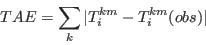
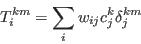
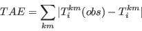
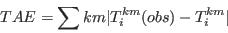
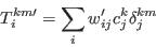
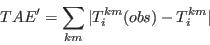
- For the purpose of this research and simplicity of interpretation, this study employs statistics based on the Total Absolute Error (TAE) statistic, defined in equation (2). The TAE calculates the number of people in the population that have been misclassified (Voas and Williamson 2001). It is expressed as
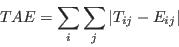
(2) where Tij and Eij are the observed and expected counts respectively for the cell at ij (here, a cell is taken to mean an item of data in a table). The advantages to using this measure are its simplicity of calculation and interpretation. However TAE can be misleading. When evaluating the degree of error in a category for a particular attribute, the raw TAE provides a figure that relates to the actual number of the population misclassified. When using the raw TAE calculation across all the categories for an attribute it is possible to produce figures larger than the population. Each misclassification event is counted twice, once when the person is omitted from a category and once when they are added to a category where they do not belong.
- 4.3
- Considering this limitation with the TAE statistic, some simple modifications have been made to facilitate interpretation of results. When considering a single cell within an attribute the raw TAE is used. Even with a maximum error the TAE will equal the expected population and not exceed it. For the same reason, when considering the error calculations for attributes where multiple categories or cells are involved, the statistic TAE/2 is adopted. Both these statistics are referred to as the Classification Error (CE); they show the number of individuals that have been misclassified in a cell, zone or attribute. It is important to note that the CE statistic is an absolute measure of misclassification and as noted by Voas and Williamson (2001) absolute measures of fit are subject to the population size. Therefore, the percentage Classification Error (% CE) is also utilised. This is a relative measure derived by CE/N where N is the population of the relevant cell, zone or attribute as appropriate. A more detailed consideration of the pros and cons of different goodness of fit tests can be found in Voas and Williamson (2001).
Results
-
Representing Constraint Variables
- 5.1
- Voas and Williamson (2000) stated that all constraint attributes should be well represented in a synthetic population. The purpose of this test is to evaluate how well the constraint attributes are reproduced in each of the algorithms. Populations are synthesised using each algorithm at each spatial scale OA, LLSOA and MLSOA, making a total of nine different synthetic populations being evaluated.
- 5.2
- Table 3 shows that only simulated annealing has successfully recreated all of the constraint attributes at all three spatial scales with zero misclassification. The conditional probabilities algorithm produces a reasonable fit for all of the constraints over each scale. However, the classification error almost doubles for each constraint as the geographical scale becomes finer. The deterministic reweighting method produced the worst fit. With the exception of Highest Qualification (which shows a slight decrease in CE, but overall this constraint has a very poor fit to the observed data) all of the constraints show a slight increase in CE as geographical scale becomes finer.
Table 3: Representation of the model constraints in the synthesised populations Constraint DR CP SA CE % CE CE % CE CE % CE Middle Layer Super Output Area Gender 29,510 4.12 102 0.01 0 0.00 Ethnic Group 14,897 2.08 2,290 0.32 0 0.00 Age 128,999 18.03 144 0.02 0 0.00 Marital Status 95,335 13.33 478 0.07 0 0.00 NSSEC 84,731 11.84 4,378 0.61 0 0.00 Highest Qualification 229,407 32.07 2,569 0.36 0 0.00 Lower Layer Super Output Area Gender 30,297 4.23 176 0.02 0 0.00 Ethnic Group 15,631 2.18 4,010 0.56 0 0.00 Age 131,230 18.34 245 0.03 0 0.00 Marital Status 96,453 13.48 842 0.12 0 0.00 NSSEC 88,282 12.34 9,659 1.35 0 0.00 Highest Qualification 228,425 31.93 5,219 0.73 0 0.00 Output Area Gender 33,430 4.67 245 0.03 0 0.00 Ethnic Group 16,707 2.34 5,292 0.74 0 0.00 Age 135,673 18.96 418 0.06 0 0.00 Marital Status 98,696 13.80 1,828 0.26 0 0.00 NSSEC 95,117 13.30 21,939 3.07 0 0.00 Highest Qualification 227,720 31.83 11,385 1.59 0 0.00 DR = deterministic reweighting, CP = conditional probabilities, SA = simulated annealing - 5.3
- To investigate the poor fit of the deterministic reweighting algorithm, the number of misclassified people per zone is plotted for the Ethnic Group, Gender and Marital Status constraints at the MLSOA geography (Figure 2–Figure 4). The Ethnic Group scatter plot (Figure 2) shows that, despite having almost 15,000 classification errors, the spread of error tracks the line of perfect fit (where each point would reside if the synthesised population matched the observed population exactly). Only small discrepancies exist, but the discrepancies are evident in many geographical zones.
- 5.4
- Figure 3 shows a scatter plot of gender classification errors which are grouped very tightly together. The lack of spread along the line of perfect fit is a reflection that most geographical zones have a relatively balanced population between male and female and do not display the extremes that can be observed in other constraint attributes. Despite the relatively ubiquitous nature of the attribute, many of the geographical zones are some distance away from the perfect fit line; this is reflected in the 29,510 classification errors observed at the MLSOA geography. This high level of error may be due to the constraint being last in the processing order and the attempt of the algorithm to smooth towards the global mean.
The marital status constraint is particularly poorly fit by the deterministic reweighting routine. Although this constraint does not have the highest level of associated classification error, it does display a distinct pattern. Most MLSOA zones have the married category over represented and the single category underrepresented in the synthetic population. This suggests that the algorithm is smoothing towards the distribution of the sample population rather than preserving the distribution observed in the constraint information for each geographical area.
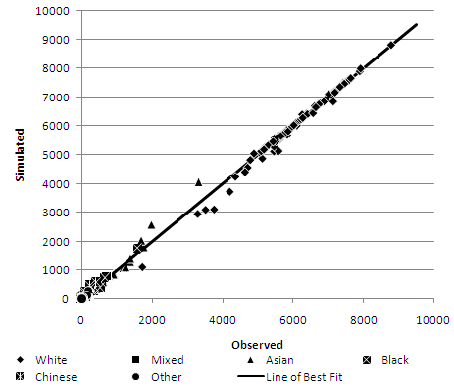
Figure 2. Deterministic reweighting - Ethnic Group misclassification error at MLSOA geography 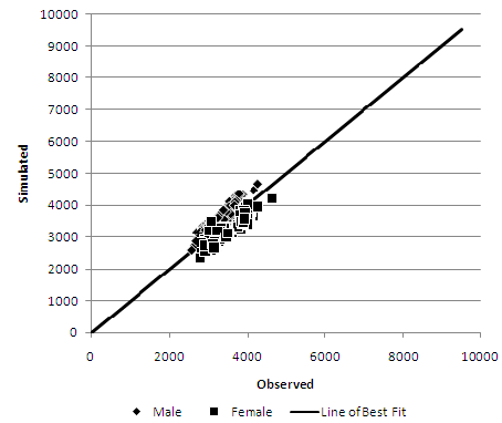
Figure 3. Deterministic reweighting - Gender misclassification error at MLSOA geography 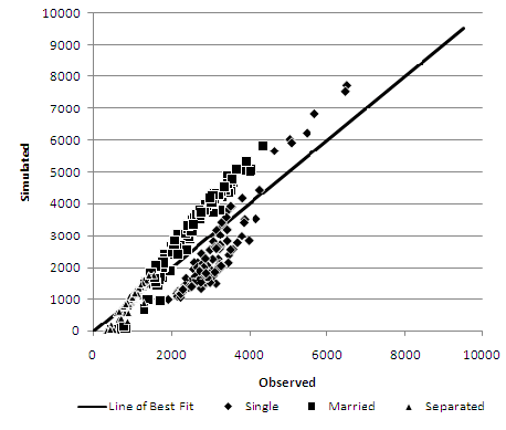
Figure 4. Deterministic reweighting - Marital Status misclassification error at MLSOA geography Recreating Observed Relationships
- 5.5
- This experiment considers how well the synthetic populations recreate observed relationships between attributes not explicitly contained in the constraints used, but implicitly contained in the sample population. The results in Table 4 show that the overall performance of the conditional probabilities and simulated annealing models are very similar, although the lowest CE and %CE is always generated by simulated annealing except for Gender by Age at the OA geography. The results of the deterministic reweighting algorithm are substantially worse.
- 5.6
- Overall, the results improve with a coarser geographical scale; LLSOA is better than OA and MLSOA better than LLSOA. This is due to larger geographical areas containing higher population numbers, and therefore a higher possibility of containing a more representative sample of the population. A result of note is the cross tabulation of Gender by Marital Status by Age. This cross-tabulation shows the worst fit for both simulated annealing and conditional probabilities approaches at the finer OA geography but is better represented than Age by Ethnic Group at the MLSOA geography. Both these cross-tabulations perform similarly under the deterministic reweighting approach. The consistently worst performing inter-constraint relationship for the deterministic reweighting approach is NSSEC by Qualification. This in itself is unsurprising as Highest Qualification is the poorest fit of the univariate constraint attributes for this method.
As an example, age scatterplots for the Pakistani ethnic group are presented in Figures 5–7. The Pakistani ethnic group is the largest, and therefore arguably the most important, of the ethnic minority groups in the Leeds area (Phillips 2004). The deterministic reweighting approach (Figure 5) shows the least consistency with a tendency to over represent the Pakistani ethnic group in areas where they have significant numbers, especially in ages from 5 to 49. Both conditional probabilities (Figure 6) and especially the simulated annealing model (Figure 7) show a much tighter distribution around the perfect fit line.Table 4: Representation of inter-attribute relationships in each synthesised population Evaluation Attributes DR CP SA CE % CE CE % CE CE % CE Middle Layer Super Output Area Age by Ethnic Group 137,177 19.17 41,300 5.77 40,179 5.62 Marital Status by Age 134,341 18.78 26,178 3.66 24,113 3.37 NSSEC by Age 104,108 14.55 15,808 2.21 14,619 2.04 NSSEC by Qualification 183,765 25.69 27,915 3.90 27,292 3.81 Gender by Age 134,281 18.77 28,159 3.94 27,228 3.81 Gender by Ethnic Group 42,984 6.01 8,537 1.19 8,328 1.16 Gender by Marital Status by Age 137,631 19.24 37,495 5.24 35,388 4.95 Lower Layer Super Output Area Age by Ethnic Group 146,431 20.47 54,369 7.60 52,503 7.34 Marital Status by Age 140,344 19.62 40,364 5.64 38,606 5.40 NSSEC by Age 109,901 15.36 27,879 3.90 24,117 3.37 NSSEC by Qualification 188,669 26.37 48,884 6.83 46,404 6.49 Gender by Age 139,753 19.53 45,180 6.32 44,380 6.20 Gender by Ethnic Group 46,937 6.56 15,748 2.20 15,035 2.10 Gender by Marital Status by Age 147,386 20.60 62,088 8.68 60,276 8.43 Output Area Age by Ethnic Group 161,688 22.60 74,463 10.41 73,100 10.22 Marital Status by Age 157,753 22.05 72,564 10.14 71,134 9.94 NSSEC by Age 123,852 17.31 53,905 7.53 45,193 6.32 NSSEC by Qualification 210,203 29.38 96,781 13.53 91,981 12.86 Gender by Age 156,148 21.83 84,661 11.83 85,097 11.89 Gender by Ethnic Group 56,115 7.84 28,013 3.92 26,560 3.71 Gender by Marital Status by Age 175,524 24.54 117,928 16.48 117,130 16.37 DR = deterministic reweighting, CP = conditional probabilities, SA = simulated annealing 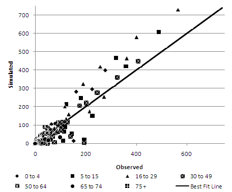
Figure 5. Deterministic reweighting at MLSOA geography - Age by Pakistani Ethnic Group 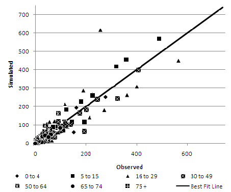
Figure 6. Conditional probabilities at MLSOA geography - Age by Pakistani Ethnic Group 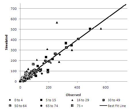
Figure 7. Simulated Annealing at MLSOA geography - Age by Pakistani Ethnic Group - 5.7
- Interestingly, the same major outlier recurs in both the conditional probabilities and the simulated annealing method. This zone is an area (Harehills / Chapeltown) which has both high ethnic concentration, but also very high student numbers. In this area, the Pakistani ethnic group makes up 67% of the 0 to 4, 45% of the 4 to 15, 22% of the 30 to 49 age groups. In contrast, the Pakistani population is vastly underrepresented at ages 16 to 29 comprising only 5% of this cohort. Overall, however, over 60% of the population of this MLSOA consists of white 16 to 29 year olds. In fact, the 16 to 29 age group is vastly over represented by the white host population which makes up over 82% of this age category but less than, and in most cases substantially less than, 53% of all other age categories.
- 5.8
- The conditional probabilities and simulated annealing algorithms are attempting to replicate the extreme anomaly of a high Pakistani population combined with a high, predominantly white student population. However, the two algorithms main source of information for the interrelationship between age and ethnic origin is from the sample information in the sample population, which represents the average distribution for the whole Leeds MDA. Thus, sampling from this district 'average' sample population has the effect of flattening out the extreme demographic observed in this particular MLSOA resulting in an overestimation of the Pakistani 16 to 29 age group.
Estimation of Unknown Attributes
- 5.9
- An increasing application of spatial microsimulation is the linkage of complicated datasets where there is no apparent join, or for the estimation of attributes that do not form part of the initial model configuration. This test examines how well each of the approaches adopted in this work can represent attributes not included in their configuration.
- 5.10
- The following attributes were utilised to test the performance of each approach. Gender by Hours Worked assesses how well the representation of a relationship to an attribute is incorporated through a cross-tabulated relationship when only one of the attributes, in this case Gender, forms part of the model configuration. Economic Activity by Car Ownership is used to evaluate the ability of the approaches to replicate an inter-attribute relationship when neither of the attributes are included in the model configuration. Finally, Long Term Limiting Illness and Tenure of Accommodation provide insights into how well univariate attributes not included in the model configuration are recreated.
- 5.11
- Table 5 contains the misclassification information for the attributes not used to constrain the model. All of the algorithms consistently perform better for at least one of the attributes than the alternative two algorithms. For Economic Activity by Car Ownership and Gender by Hours Worked, the simulated annealing algorithm consistently produces the best result at all spatial resolutions. The Limiting Long Term Illness attribute is best estimated by the conditional probabilities algorithm and Tenure of Accommodation is estimated most accurately by the deterministic reweighting algorithm. It is noteworthy that the simulated annealing algorithm has been outperformed at estimating both of the univariate attributes not contained in the model configuration by the other algorithms. These results, and those from ¤5.5, suggest that the simulated annealing algorithm is the most reliable at recreating the observed relationships between attributes. When comparing the results between Gender by Hours Worked and Economic Activity by Car Ownership, all three models produced a more accurate fit when a known attribute was included in the model configuration.
Table 5: Extent of attribute capture outside of the constraint attributes
Unknown AttributesDR CP SA CE % CE CE % CE CE % CE Middle Layer Super Output Area Economic Activity by Car Ownership 109,089 15.25 76,050 10.63 63,632 8.89 Limiting Long Term Illness 34,700 4.85 15,147 2.12 26,993 3.77 Gender by Hours Worked 63,973 8.94 24,572 3.43 15,357 2.15 Tenure of Accommodation 87,809 12.27 105,912 14.80 108,852 15.22 Lower Layer Super Output Area Economic Activity by Car Ownership 118,154 16.52 90,278 12.62 77,138 10.78 Limiting Long Term Illness 35,753 5.00 16,903 2.36 26,703 3.73 Gender by Hours Worked 67,425 9.42 29,707 4.15 22,714 3.17 Tenure of Accommodation 114,431 16.00 133,277 18.63 135,860 18.99 Output Area Economic Activity by Car Ownership 140,762 19.68 119,018 16.64 106,400 14.87 Limiting Long Term Illness 38,845 5.43 23,357 3.26 30,085 4.21 Gender by Hours Worked 79,041 11.05 46,104 6.44 40,939 5.72 Tenure of Accommodation 142,566 19.93 160,363 22.42 163,904 22.91 DR = deterministic reweighting, CP = conditional probabilities, SA = simulated annealing - 5.12
- Comparing the estimation of the two univariate attributes, Limiting Long Term Illness is less affected by spatial location; it is more likely to be a product of the working environment than of the home one with all sections of society being exposed to illnesses such as stress. Tenure of Accommodation has more of an explicit spatial pattern. Typically, higher concentrations of home owner are located in suburbs, with young professionals renting in city centres, producing a spatial disparity to the distribution of home owners and renters from the same socio-economic group. This suggests that the ability to tailor the deterministic reweighting algorithm through the application of different constraint orders for geographical zones with similar attributes may provide more satisfactory results when considering a spatially disparate attribute.
- 5.13
- Furthermore, Limiting Long Term Illness has less correlation to the attributes used to constrain the model with only one significant correlation coefficient of 0.60 to persons of pensionable age (over 65). In comparison Tenure of Accommodation is significantly correlated to middle-aged persons (40 - 65) with a coefficient of 0.80, single people (0.89) and higher NSSEC groups (0.86). Subsequently, one would expect Tenure of Accommodation to be the more accurately replicated result. However, despite having a distinctively more defined relationship to attributes contained in the model constraints, the Tenure of Accommodation attribute is the less well represented of the two. This is due to the distribution of Tenure of Accommodation categories in the sample population. The overall distribution of home owners observed in the Leeds area is 65% which is consistent with the distribution of home owners in the total sample population used to synthesise the population. However, the distribution of homeowners in the sample population reduces to 56% when the sample population is filtered to the constraint attributes that are highly correlated to the Tenure of Accommodation attribute. This results in both spatial disparity and a sampling bias in the Tenure of Accommodation attribute and highlights that, despite Tenure of Accommodation being highly correlated to attributes included in the model configuration, it does not necessarily follow that this attribute will be estimated with a high degree of accuracy.
Aggregation of Outputs
- 5.14
- Deterministic reweighting is partially dependant on the clustering of zones into similar groups to enable effective constraint configuration. Therefore, deterministic reweighting is disadvantaged when considering LLSOA and MLSOA geographies because of the limited number of zones available to the clustering routine. To provide a fair evaluation of the performance of the methods, the output at OA level, where effective zone clustering can be achieved, is aggregated to LLSOA and MLSOA.
- 5.15
- Tables 6 and 7 present the resulting misclassification errors for the OA geographies once aggregated to LLSOA and MLSOA. The aggregated results show a negligible difference in performance to those produced in the previous sections at the LLSOA and MLSOA geographies for the simulated annealing and conditional probabilities methods. The variation in results can be attributed to the stochastic nature of these two models rather than performing more effectively at a particular geography. Furthermore, the absence of a significant improvement in reproduction of attributes when aggregating from a finer geographic scale as opposed to generating the results directly at the spatial scale in question, indicates that spatial scale is less important than the variability of the attributes over the spatial scale with respect to the accuracy with which attributes are reproduced.
Table 6: OA results aggregated to MLSOA
ConstraintDR CP SA CE % CE CE % CE CE % CE Constraints Gender 26,722 3.74 141 0.02 0 0.00 Ethnic Group 13,305 1.86 2,054 0.29 0 0.00 Age 112,520 15.73 363 0.05 0 0.00 Marital Status 83,989 11.74 564 0.08 0 0.00 NSSEC 71.939 10.06 5,856 0.82 0 0.00 Highest Qualification 213,389 29.83 2,514 0.35 0 0.00 Inter-constraint cross tabulations Age by Ethnic Group 121,220 16.94 40,596 5.67 38,914 5.44 Marital Status by Age 118,832 16.61 25,447 3.56 23,636 3.30 NSSEC by Age 89,165 12.46 16,583 2.32 13,805 1.93 NSSEC by Qualification 171,335 23.95 28,064 3.92 26,179 3.66 Gender by Age 118,964 16.63 27,317 3.82 27,110 3.79 Gender by Ethnic Group 39,102 5.47 8,565 1.20 7,717 1.08 Gender by Marital Status by Age 123,161 17.22 36,400 5.09 34,623 4.84 External attribute representation Economic Activity by Car Ownership 97,820 13.67 76,084 10.64 62,202 8.69 Limiting Long Term Illness 35,739 5.00 15,835 2.21 26,603 3.72 Gender by Hours Worked 56,813 7.94 25,534 3.57 15,523 2.17 Tenure of Accommodation 91,193 12.75 105,705 14.78 108,885 15.22 DR = deterministic reweighting, CP = conditional probabilities, SA = simulated annealing Table 7: OA results aggregated to LLSOA Constraint DR CP SA CE % CE CE % CE CE % CE Constraints Gender 28,438 3.98 205 0.03 0 0.00 Ethnic Group 14,755 2.06 3,455 0.48 0 0.00 Age 120,644 16.86 406 0.06 0 0.00 Marital Status 88,157 12.32 966 0.14 0 0.00 NSSEC 79,472 11.11 10,827 1.51 0 0.00 Highest Qualification 217,702 30.43 5,317 0.74 0 0.00 Inter-constraint cross tabulations Age by Ethnic Group 136,123 19.03 53,300 7.45 51,763 7.24 Marital Status by Age 130,554 18.25 39,512 5.52 38,237 5.34 NSSEC by Age 99,611 13.92 28,222 3.94 23,918 3.34 NSSEC by Qualification 180,030 25.16 48,412 6.77 45,651 6.38 Gender by Age 129,991 18.17 44,465 6.22 44,230 6.18 Gender by Ethnic Group 44,434 6.21 15,529 2.17 14,661 2.05 Gender by Marital Status by Age 138,136 19.31 60,747 8.49 59,837 8.36 External attribute representation Economic Activity by Car Ownership 110,796 15.49 90,902 12.71 76,531 10.70 Limiting Long Term Illness 36,390 5.09 17,549 2.45 27,013 3.78 Gender by Hours Worked 62,319 8.71 30,696 4.29 22,621 3.16 Tenure of Accommodation 116,417 16.27 133,053 18.60 135,636 18.96 DR = deterministic reweighting, CP = conditional probabilities, SA = simulated annealing - 5.16
- However, the deterministic reweighting algorithm does show some improvement in performance when first run at the finer OA spatial scale, and then aggregated. A great advantage of this model is the clustering of similar zones by characteristics and then configuring the model to use the best constraint order for those zones, providing a much better spatial representation for attributes. When using coarse geographical zones the clustering routines and constraint ordering become less effective and influential; this results in a poorer performing model. It must be noted that although the deterministic reweighting algorithm improves in performance at a finer geographic scale, the results still do not rival that of the other two techniques, with the exception of when significant spatial disparities are evident in an attribute.
Conclusions
- 6.1
- The work in this paper has examined the performance of deterministic reweighting, conditional probabilities and simulated annealing spatial microsimulation methods for generating synthetic populations over varying spatial scales. Of the three methods assessed, simulated annealing was found to consistently produce the best outcome when fitting constraints. $5.1 demonstrated that the deterministic reweighting algorithm tends to smooth towards the sample mean rather than preserving the peculiarities of each individual zone. This could be due to the lack of a method for this algorithm to reweight probabilities (in the case of conditional probabilities method) or to try new population configurations in the case of simulated annealing. Both of these algorithms automatically adjust to under and over projections to some extent, whereas the deterministic reweighting algorithm iteratively smooths the weights towards the distribution observed in the sample population.
- 6.2
- When considering the recreation of relationships between attributes in ¤5.5, the summary statistics reveal that the simulated annealing algorithm slightly outperforms the conditional probabilities algorithm and both outperform the deterministic reweighting approach. However, when examining zones where extreme differences in the observed population in the zone and the sample population are present, such as the one exemplified in Harehills and Chapeltown, the simulated annealing and conditional probabilities methods are limited to the extent that inter-attribute relationships can be replicated using the inter-relationship information from the sample population. This problem could be overcome by incorporating critical inter-attribute relationship information in the model specification, and is therefore a limitation of model specification rather than an algorithmic defect.
- 6.3
- On the basis of this work, several recommendations for optimal performance can be made. Including the cross tabulation of a constraint or a highly correlated variable in the model configuration when attempting to predict an unknown attribute improves the result. The spatial scale at which a population is generated is less important for the conditional probabilities and simulated annealing methods than the spatial variability of any attributes that are to be predicted / simulated. The deterministic reweighting algorithm performs much better at finer geographic scales, where clustering and constraint configuration techniques are more effective.
- 6.4
- Related to this, the simulation of attributes that are particularly influenced by spatial locations is best undertaken using the deterministic reweighting algorithm. This method allows the constraint order to be tailored to best represent a particular cluster of zones and is more accurate when the purpose is to model one distinct outcome, such as smoking, rather than recreating a generic population (Smith et al. 2011; Tomintz et al. 2008). Although, it may be possible to design a more intelligent search algorithm for the simulated annealing approach to enhance the capability of this algorithm to capture an attributes spatial variability.
- 6.5
- As highlighted in ¤5.9, spatial variability and the level of correlation to constraint attributes are not the only determinants for whether a non-constraining attribute can be well represented. Sampling bias can have a significant impact on the representation of the attribute and it may well be that a more established statistical modelling process such as multiple regression could be applied with greater success in these situations.
- 6.6
- On the whole, the simulated annealing algorithm outperformed both deterministic reweighting and conditional probabilities algorithms, although only marginally in some cases. It could be argued that the marginally better results of the simulated annealing approach over the conditional probabilities method could be outweighed by the quicker execution time of the conditional probabilities method. However, the quicker execution speed of the conditional probabilities method is offset by additional analysis required pre-model run to determine the best order of constraints. It is hard to advocate one method as the clear 'winner', each algorithm has advantages and disadvantages, and each maybe more suited to particular projects. However, simulated annealing does hold great potential, and with computing power ever increasing the computationally intensive nature of the algorithm is becoming less of a hindrance.
- 6.7
- One area of great potential for this work is the linkage of these synthesised populations to other techniques now being widely used in social science simulation, in particular, agent-based modelling. Realistic individual-level populations can be generated that mimic specific characteristics about a geographical area, or a specific application; for example, populations can be generated that contain characteristics of particular interest to health or education researcher. These populations can be turned into individual agents that form part of a larger modelling effort. The work of Wu and Birkin (2012) and Harland and Heppenstall (2012) hint at the possibilities that customised individual-level agent populations can bring to this area of research.
Notes
-
1In which examples of attributes would be age, gender, ethnicity and so on. If the attribute is ethnicity, then the characteristics might be White British, Asian, or Caribbean.
Suggested Further Readings
-
Synthetic population creation, including multilevel methods:
TWIGG, L. & Moon, G. (2002). Predicting small area health-related behaviour: a comparison of multilevel synthetic estimation and local survey data. Social Science & Medicine, 54, 931-937.MOON, G., Quarendon, G., Barnard, S., Twigg, L., & Blyth, B. (2007). Fat nation: Deciphering the distinctive geographies of obesity in England. Social Science & Medicine, 65, 25-31.
PEARCE, J., Boyle, P., & Flowerdew, R. (2003). Predicting smoking behaviour in census output areas across Scotland. Health & Place, 9, 139-149.
Microsimulation:
TANTON, R., Vidyattama, Y., Nepal, B., & McNamara, J. (in press). Small area estimation using a reweighting algorithm. Journal of the Royal Statistical Society: Series A.
WILLIAMSON, P., Birkin, M., & Rees, P.H. (1998). The estimation of population microdata by using data from small area statistics and samples of anonymised records. Environment and Planning A, 30, 785-816.
MERZ, J. (1991). Microsimulation - A survey of principles, developments and applications. International Journal of Forecasting, 7, 77-104.
Deterministic reweighting:
ANDERSON, B. (2007). Creating small-area income estimates: spatial microsimulation modelling. Department for Communities and Local Government, London.
BALLAS, D., Clarke, G., Dorling, D., Eyre, H., Thomas, B., & Rossiter, D. (2005). SimBritain: A Spatial Microsimulation Approach to Population Dynamics. Population Space and Place, 11, 13-34.
DUECK, G. & Scheuer, T. (1990). Threshold Accepting: A General Purpose Optimization Algorithm Appearing Superior to Simulated Annealing. Journal of Computational Physics, 90, 161-175.
Simulated Annealing:
INGBER, L. (1993). Simulated Annealing: Practice Versus Theory. Mathematical and Computer Modelling, 18, 29-57.
KIRKPATRICK, S.; Gelatt, C. D.; and Vecchi, M. P. "Optimization by Simulated Annealing." Science 220, 671-680, 1983.
METROPOLIS, N., Rosenbluth, A. W., Rosenbluth, M., Teller, A. H., & Teller, E. (1953). Equation of State Calculations by Fast Computing Machines. Journal of Chemical Physics, 21, 1087-1092.
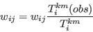
Appendix A: The problem expressed mathematically
- A.1
- To express the modelling problem in mathematical terms, the characteristics of the individuals in the sample population can be expressed as:
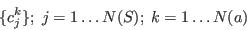
where N(S) is the number of individuals in the sample; N(a) is the number of attributes in the model; and cjk is therefore the characteristic of attribute k in the jth member of the population sample.
- A.2
- The weights are given simply as:
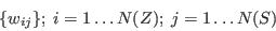
where N(Z) is the number of small areas (zones) in the study region.
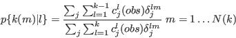
- A.3
- The cells in the constraining tables are:

in which we use the postscript 'obs' as a convention to distinguish an observed count of the number of individuals in area i with characteristic m for attribute k (so that in the case the unadorned 'Tikm' would represent a model-based estimate of the same cells). For the purposes of this discussion we will assume that the attributes in the constraining table are uni-dimensional, although this assumption can be relaxed without any significant impact on the modelling process.
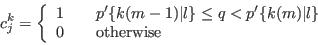
- A.4
- The individual modelled elements of the constraint vector can be estimated as:
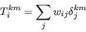
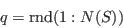
in which the binary variable δjkm takes the value of one if cjk = m, and zero otherwise. In order to compare the modelled and observed distributions, a variety of goodness of fit measures could be employed, but typically the most useful will be the total absolute error statistic:
Appendix B: Deterministic Reweighting in Spatial Microsimulation
- A.5
- Step 1 - Initialise the weights

- A.6
- Step 2 - Implement the algorithm for each of the attributes in turn

- A.7
- Step 3 - Generate cell counts from the model using the current weights
- A.8
- Step 4 - Update the weights based on the comparison between the model cell counts and the constraining tables
- A.9
- Step 5 - Repeat steps 2 to 4 until there is no further reduction in the total absolute error:

Appendix C: Conditional Probabilities
- A.10
- Step 1 - Implement the algorithm for each of the attributes in turn

- A.11
- Step 2 - Initialise the weights for the current attribute

- A.12
- Step 3 - Compute conditional probabilities from all the attributes so far established
- A.13
- Step 4 - Assign synthetic characteristics from cumulative conditional probabilities:


- A.14
- Step 5 - Adjust weights to balance constraining tables

- A.15
- Step 6 - Iterate through steps 3 to 5 until there is no further reduction in the Total Absolute Error:
Appendix D: Simulated Annealing
- A.16
- Step 1 - Configure the temperature steps - starting value of t0 and steps of t (t0 >> t)
- A.17
- Step 2 - Generate a random solution
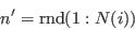
- Set all weights to zero and initialise counters:

- Select individuals at random:


- Repeat step (ii) until the required number of individuals has been selected:

- Set all weights to zero and initialise counters:
- A.18
- Step 3 - Compute goodness of fit for the current solution

- A.19
- Step 4 - Replace one individual at random
- From the current selection, pick an individual and flip the weight from 1 to 0:


- Pick a new individual at random from the sample:
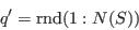


- From the current selection, pick an individual and flip the weight from 1 to 0:
- A.20
- Step 5 - Calculate the goodness of fit for the new solution:
- A.21
- Step 6 - Update the weights if the annealing threshold is exceeded:

- A.22
- Step 7 - Repeat steps 3 to 6 until the annealing threshold is zero:

Appendix E: Maps showing the different geographical layers within the study area
Acknowledgements
- This work forms part of the ESRC funded Modelling Individual Consumer Behaviour project (RES-061-25-0030). Part of this work was funded by a Royal Geographical Society small grants award (SRG 04/09) and an MRC Population Health Scientist Fellowship (G0802447).
References
-
ANDERSON, B. (2007). Creating small-area Income Estimates: spatial microsimulation modelling, Department for Communities and Local Government, Communities and Local Government Publications, London.
BALLAS D., Clarke, G., Dorling, D., Eyre, H., Thomas, B., & Rossiter D. (2005). SimBritain: a spatial microsimulation approach to population dynamics. Population, Space and Place, 11, 13-34. [doi:10.1002/psp.351]
BECKMAN, R. J., Baggerly, K. A ., & McKay, M. D. (1996). Creating synthetic baseline populations. Transportation Research, 30, 415-429.
BIRKIN, M. & Clarke, M. (1988). SYNTHESIS - a synthetic spatial information system for urban and regional analysis: methods and examples'' Environment and Planning A, 20, 1645 -1671. [doi:10.1080/00343408912331345702]
BIRKIN, M. & Clarke, M. (1989).The generation of individual and household incomes at the small area level using synthesis'' Regional Studies, 23, 535 - 548. [doi:10.1080/00343408912331345702]
BROWN, L., & Harding, A. (2002). Social modelling and public policy: Application of microsimulation modelling in Australia. Journal of Artificial Societies and Social Simulation, 5(4) 6. http://jasss.soc.surrey.ac.uk/5/4/6.html
DAVIES, L. (1987). Genetic algorithms and simulated annealing. Research Notes in Artificial Intelligence. Los Altos, CA: Morgan Kaufmann.
HARLAND, K. & Heppenstall, A.J. (2012). Using Agent-Based Models for Education Planning: Is the UK Education System Agent-Based. In Heppenstall, A.J., Crooks, A.T., See, L.M., & Batty, M. (Eds.) Agent-based models of Geographical Systems. Dordrecht: Springer. [doi:10.1007/978-90-481-8927-4_23]
HEPPENSTALL, A.J., Evans, A.J., Birkin, M.H. (2006). Application of multi-agent systems to modelling a dynamic, locally interacting retail market. Journal of Artificial Societies and Social Simulation, 9(3)2. http://jasss.soc.surrey.ac.uk/9/3/2.html
HEPPENSTALL, A.J., Crooks, A.T., See, L.M., & Batty, M. (Eds.) (2012). Agent-Based Models of Geographical Systems. Dordrecht: Springer.
MALLESON, N.S., Heppenstall, A.J., & See, L.M. (2010). Simulating burglary with an agent-based model. Computers, Environment and Urban Systems 31(3) 236-250. [doi:10.1016/j.compenvurbsys.2009.10.005]
MCFADDEN, D., Cosslett, S., Duguay, G. & Jung, W. (1977). Demographic Data for Policy Analysis. Urban Travel Demand Forecasting Project, Final Report Series, Vol VIII. University of California, Berkeley and Irvine: Institute of Transportation Studies.
MORRISSEY, K., Clarke, G., Ballas, D., Hynes, S., & O'Donoghue, C. (2008). Examining access to GP services in rural Ireland using microsimulation analysis. Area, 40, 354-364. [doi:10.1111/j.1475-4762.2008.00844.x]
OPENSHAW, S. & Rao, L. (1995). Algorithms for reengineering 1991 Census geography. Environment and Planning A, 27, 425-446. [doi:10.1068/a270425 ]
OTTEN, R.H.J.M. & van Ginneken, L.P.P.P. (1989). The Annealing Algorithm: The Springer International Series in Engineering and Computer Science. Boston, MA: Kluwer.
PHILLIPS, D. (2004). Mulitcultural Leeds: Geographies of ethnic minorities and religious groups. In Twenty-first century Leeds: Geographies of a regional city. Unsworth, R. & Stillwell, J.C.H. (Eds.). Leeds: Leeds University Press.
SMITH, D.M., Clarke, G.P., & Harland, K. (2009). Improving the synthetic data generation process in spatial microsimulation models. Environment and Planning A, 41, 1251 - 1268. [doi:10.1068/a4147]
SMITH, D.M., Pearce, J.R., & Harland, K. (2011). Can a deterministic spatial microsimulation model provide reliable small-area estimates of health behaviours? An example of smoking prevalence in New Zealand. Health & Place, 17, 618-624. [doi:10.1016/j.healthplace.2011.01.001]
STILLWELL, J.C.H. & Duke-Williams, O. (2002). A new web-based interface to GB Census of Population origin-destination statistics. Environment and Planning A, 35, 113 -132. [doi:10.1068/a35155]
TOMINTZ, M.N., Clarke, G.P., & Rigby, J. (2008). The geography of smoking in Leeds: estimating individual smoking rates and the implications for the location of stop smoking services. Area, 40,341-353. [doi:10.1111/j.1475-4762.2008.00837.x]
VOAS, D. & Williamson P. (2000). An evaluation of the combinatorial optimisation approach to the creation of synthetic microdata. International Journal of Population Geography,6, 349 - 366. [doi:10.1002/1099-1220(200009/10)6:5<349::AID-IJPG196>3.0.CO;2-5]
VOAS, D. & Williamson, P. (2001). Evaluating goodness-of-fit measures for synthetic microdata. Geographical and Environmental Modelling, 5, 177 - 200. [doi:10.1080/13615930120086078]
WILLIAMSON, P., Birkin, M., & Rees, P. (1998). The estimation of population microdata by using data from small area statistics and samples of anonymised records. Environment and Planning A, 30, 785 - 816. [doi:10.1068/a300785 ]
WILLIAMSON, P. & Clarke, G.P. (1996). Estimating small-area demands for water with the use of microsimulation. In Microsimulation for urban and regional policy analysis. Clarke, GP (Ed.). London: Pion.
WU, B.M. & Birkin, M.H. (2012), Agent-based Extensions to a Spatial Microsimulation Model of Demographic Change. In Agent-based models of Geographical Systems. Heppenstall, A.J., Crooks, A.T., See, L.M. & Batty, M. (Eds.) Dordrecht: Springer.